Notes on Q learning

• Introduction
  • Reinforcement Learning Basic Setup
  • State Value and Action Value
  • Model Based Vs Model Free
  • On Policy Vs Off Policy Methods
  • Temporal difference Learning
• Q-Learning:
  • The Q learning Algorithm
  • Q Learning Vs SARSA:
    • SARSA
    • The sarsa Algorithm
• Case Study : Cliff Walker Enviornment
  • Policy Comparision
• Summary
• Useful resources

Introduction

Q learning is one of the sucessful techniques in Reinforcement Learning .It was initially introduced in 1989 by Watkins. Q learning came to light when Deepmind used it to play Atari games with superhuman perfomance in 2015.

In General,Q learning is a model free learning .Its an off policy TD Control.

In this post , We will see a small RL Introduction , then into Qlearning and end with Qlearning & Sarsa Comparision.

The jupyter notebook comparision of Q learning and SARSA for the cliff walker enviornment can be found here.

Reinforcement Learning Basic Setup

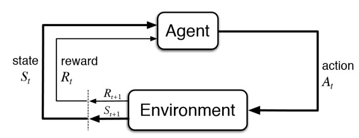
Simply , In Reinforcement Learning, the Agent acts on the Enviornment with Action and collects the Reward. The Enviornment transitions from an older state to a new state in reponse to the action by the Agent.

State Value and Action Value

Policy defines the learning agents way of behaving at a given time.A policy is a Mapping from States to probability of selecting different actions.Its denoted by $\pi$.

If the agent is following policy $\pi$ at time t , then $\pi(a\mid s)$ is the probability that action $A_{t}$ = a if state,$S_{t}$ =s.

Reward is the goal of the RL Problem. The objective of the agent is to maximize the total rewards over time.

The State Value for a state $s$ under policy $\pi$ denoted as $v_{\pi}(s)$ ,is defined as the Expected return when starting in $s$ and following policy $\pi$ thereafter.

$v_{\pi}(s) = \mathbb{E}_{\pi} \left[ G_{t} | S_{t}=s \right] = \mathbb{E}_{\pi}\left[ \sum_{k=0 }^{\infty}\gamma^{k}R_{t+k+1}|S_{t}=s \right]$

for all s $\in$ S.

The value of the state is the total amount of reward which the agent can accumulate over time. Each state s has a value v(s) .

State	Value
State1	$v(s1)$
State2	$v(s2)$
State3	$v(s3)$
State4	$v(s4)$

Action value denoted as $Q(s,a)$ is the expected return starting from state s, taking an action a and then following policy $\pi$.

$q_{\pi}(s,a) = \mathbb{E}_{\pi} \left[ G_{t} | S_{t}=s ,A_{t}=a \right] = \mathbb{E}_{\pi}\left[ \sum_{k=0 }^{\infty}\gamma^{k}R_{t+k+1}|S_{t}=s ,A_{t}=a \right]$

We have qvalues for each state for all the possible actions .

Lets say , we have four states and each state has three possibe actions ,then Q values can be shown in the tabular form

State/Actions	Action1	Action2	Action3
State1	$Q(s1,a1)$	$Q(s1,a2)$	$Q(s1,a3)$
State2	$Q(s2,a1)$	$Q(s2,a2)$	$Q(s2,a3)$
State3	$Q(s3,a1)$	$Q(s3,a2)$	$Q(s3,a3)$
State4	$Q(s4,a1)$	$Q(s4,a2)$	$Q(s4,a3)$

As shown in the table above There is a action value $Q$ for all the actions in a state unlike the Value function $V$ that has a value just for each state.When the model is not available, the Q values helps to choose the next best action from that state.

Model Based Vs Model Free

Model Free means that we do not learn the model of the enviornment. We do not learn complete map of the domain. We do not learn the Probability Transition from one state to another state. $P(S^{'}| S,a)$.

Although we need a model , we need the model to generate only sample transitions, not the complete probability distributions of all possible transitions.

At the end of the learning in model free methods, we won’t have transition probabilities of the enviornment neither we know the rewards we will get without taking that action. However a policy alone is learnt based on the model(eg.Policy Gradient , Q learning)

On Policy Vs Off Policy Methods

• On-Policy methods attempt to improve the policy that is used to make decisions.
• Off-Policy methods evaluate or improve a policy different from the one that is used to make decisions.

In On-Policy methods - the Policy that is being learnt and the policy that is used to explore ,move to next state are the same.

In off policy methods, two different policies are used.

1. Target policy - The policy that is being learned about - This will be the optimal policy.
2. Behaviour policy - The policy that is used to generate behaviour - This will be more exploratory to explore more actions.

Q learning is an off policy TD control as the policy we use to estimate qvalues and the policy that is used to take actions are different.

Temporal difference Learning

TD stands for Temporal difference Learning.

TD is a hybrid of both the Montecarlo and Dynamic programming.

• Like MonteCarlo, its Model free.(ie) TD methods can learn directly from raw experience without a model of the enviornments dynamics.
• Like Dynamic Programming , they bootstrap , meaning they update estimates based on other estimate and doesn’t wait for the END of the episode to update.
• TD uses sample updates like Montecarlo

It involves

• From a state ,look ahead of the sampled sucessor state,
• Compute a Backed up value, using the value of sucessor state and the reward collected along the way ,
• Update the value of the state accordingly

The simplest TD method makes the update:

$V({S_t}) \leftarrow V({S_t}) + \alpha \left[{R_{t+1}} + \gamma V({S_{t+1}}) - V({S_t})\right]$

Here $V({S_t})$ is the estimated value and $V({S_{t+1}})$ is the successor state , ${R_{t+1}}$ is the reward collected and the computed backedup value is ${R_{t+1}} + \gamma V({S_{t+1}})$

The Error between the estimated value of $S_{t}$ and the better estimate $({R_{t+1}} + \gamma V({S_{t+1}}) - V({S_t}))$ is called TD error $\delta$.

$\delta_{t} = {R_{t+1}} + \gamma V({S_{t+1}}) - V({S_t})$

More Genericially , TD Update can be written as

$NewEstimate \leftarrow OldEstimate + stepsize \left[ Target - OldEstimate\right]$

When the model is not available we will be using Action values. (because to calculate state value, we need probability transions)

The TD(0) update for action values is :

$Q({S_t},{A_t}) \leftarrow Q({S_t},{A_t}) + \alpha \left[{R_{t+1}} + \gamma Q({S_{t+1}},{A_{t+1}}) - Q({S_t},{A_t})\right]$

Q-Learning:

Q learning is an off policy TD Control.

The equation for Q learning is

$Q({S_t},{A_t}) \leftarrow Q({S_t},{A_t}) + \alpha \left[{R_{t+1}} + \gamma \underset{a}{max} Q({S_{t+1}},a) - Q({S_t},{A_t})\right]$

In Q learning ,we force the target policy $Q(S,A)$ to move towards the optimal $q^{*}$ by acting greedily ($\underset{a}{max} Q({S_{t+1}},a)$) in that state . We dont follow that greedy action .The update is made assuming we follow the greedy behaviour.-Similiar to asking the question.. What is the estimate of $Q({S_t},{A_t})$ if we take a greedy action at this state ${S_{t+1}}$.We collect rewards $R_{t+1}$ for the initial action ${A_{t}}$ and compute the backedup action values for $Q({S_{t+1}},a)$, and use it to estimate the values at $Q({S_t})$

Since both the policies are different , Q learning is Off policy

The Q learning Algorithm

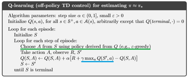
It should be clear from above that , for each estimate of Q at state $S_{t}$ , Q learning uses the maximum action value of the the state $S_{t+1}$ (Highlighted in blue).However, the next action is always derived by a different policy such as $\epsilon$-greedy (Highlighted in Green)

Q Learning Vs SARSA:

SARSA

SARSA is defined as on-policy TD Control to find optimal policy. It stands for the transition given by State,Action,Reward,(next)State,(next)Action - SARSA

The sarsa update equation is given as

$Q({S_t},{A_t}) \leftarrow Q({S_t},{A_t}) + \alpha \left[{R_{t+1}} + \gamma Q({S_{t+1}},{A_{t+1}}) - Q({S_t},{A_t})\right]$

We use the backed up action values at next state $Q({S_{t+1}},{A_{t+1}})$ to re-estimate the values at state $Q({S_t},{A_t})$

In SARSA the updates are made assuming we follow the actions defined by the policy - There is no seperate greedy policy for the updates. as in Q learning. The policy used to make the update and the one used to pick next action is the same.Thus SARSA is online.

From the state ${S_t}$,the agent chooses ${A_t}$ , collects a reward ${R_{t+1}}$ , and goes to the next state ${S_{t+1}}$. The agent chooses the next action ${A_{t+1}}$ based on its policy .We collect the action values at $Q({S_{t+1}},{A_{t+1}})$ and use it to estimate action values of the former state action $Q({S_t},{A_t})$ .

The sarsa Algorithm

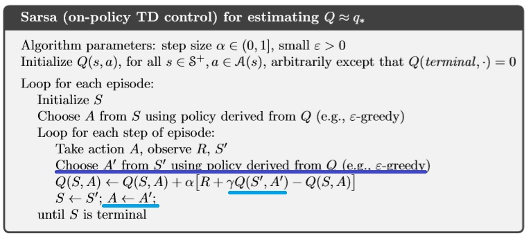
In the line highlighted with Blue, the Agent chooses an action A’ from next state state S’ state using the greedy policy to update the current state S. In the final line $A\leftarrow A^{'}$ , the same action A’ selected previously (by $\epsilon$-greedy policy) for the update is used by the Agent to transition to the next state .

Case Study : Cliff Walker Enviornment

Here we shall find a case study with Cliff Walker Enviornment . Here is the jupyter notebook comparision of Q learning and SARSA for the cliff walker enviornment.

` This is a simple implementation of the Gridworld Cliff reinforcement learning task.

Adapted from Example 6.6 (page 132) from Reinforcement Learning: An Introduction
by Sutton and Barto:
http://incompleteideas.net/book/RLbook2020.pdf

With inspiration from:
https://github.com/dennybritz/reinforcement-learning/blob/master/lib/envs/cliff_walking.py

The board is a 4x12 matrix, with (using Numpy matrix indexing):
    [3, 0] as the start at bottom-left
    [3, 11] as the goal at bottom-right
    [3, 1..10] as the cliff at bottom-center

Each time step incurs -1 reward, and stepping into the cliff incurs -100 reward
and a reset to the start. An episode terminates when the agent reaches the goal.`

The enviornment is shown below

o  o  o  o  o  o  o  o  o  o  o  o
o  o  o  o  o  o  o  o  o  o  o  o
o  o  o  o  o  o  o  o  o  o  o  o
S  C  C  C  C  C  C  C  C  C  C  G

Here,

• S is the only starting point.
• G is the Target Goal.
• C is Cliff .
• Stepping into C causes Reward to be -100.
• Stepping into C causes agent to restart from S
• Reward is -1 on on all other transitions.

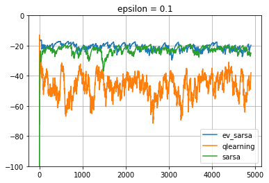
We will run both the Q learning and Sarsa on this enviornment to compare their performances.

We could see that Q learning learns the best policy after an inital transient.

Policy Comparision

The policy learnt by both the Q learning and SARSA can be compared.

Q-Learning Actions

 >  >  >  >  >  >  >  v  v  >  v  v 
 >  >  >  >  >  >  >  >  >  >  >  v 
 >  >  >  >  >  >  >  >  >  >  >  v 
 S  C  C  C  C  C  C  C  C  C  C  G

Here we can see from the starting point S, the policy goes to the immediate right and reaches the Goal.

SARSA Actions

 >  >  >  >  >  >  >  >  >  >  >  v 
 ^  ^  ^  >  >  >  >  >  >  >  >  v 
 ^  ^  ^  ^  ^  ^  ^  ^  ^  ^  >  v 
 S  C  C  C  C  C  C  C  C  C  C  G

Here we can see , the agent goes to the top of the grid , takes a right and then reaches the Goal

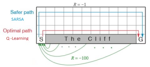
SARSA takes the longer, safer path going to the top and then moving towards the Goal. However, Q learning takes the best action and takes the path near to the cliff, the optimal path (shortest) . sarsa is an onpolicy algorithm and it cannot afford to fall the cliff every time. So it takes a much safer path.

Summary

First we saw the RL setup , some basic blocks in RL and then finally we compared Q learning with Sarsa. I just scratched the surface here.There is so much to explore in RL. I hope this will give a small boost for the beginner to dive deep to Reinforcement Learning .

Keep Learning ! Start DOING !!

Useful resources

1. Book:Reinforcement Learning An introduction by Sutton & Barto
2. OnPolicy Vs Off Policy
3. Modelbased Vs ModelFree- from Reddit
4. Modelbased Vs ModelFree- from Quora
5. RL Intro- KD Nuggets
6. Q-learning Vs SARSA
7. Distill - Understanding TD
8. RL Intro -lilianweng.github.io
9. Good RL Series by Massimiliano