An Introduction to PPO

Introduction:

PPO stands for Proximal Policy Optimization. Its a Policy gradient method for Reinforcement Learning(RL). It has much better performance than the TRPO (Trust Region Policy Optimization) but very simpler to Implement, more general and have better sample complexity.

PPO Paper: https://arxiv.org/pdf/1707.06347.pdf

Firstly, we see the basic RL setup , then explain Policy Gradients and then show the application of Importance sampling and finally the need for Policy Bounding. Basic math equations are covered as it cant be avoided altogether to understand Policy gradient and PPO .

Reinforcemet Learning Setup:

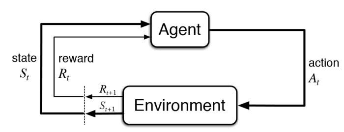
A standard RL setup consists of

• Agent
• Environment

The Agent Interacts with the Environment by taking an action and collects the rewards and observes the next state of the environment. The environment is assumed to be fully observable so that we can formulate this as Markov Decision Process.(MDP)

# This can be shown as ,
observation, reward,_ = env.step(action)

The Agent interacts with the environment in discrete timesteps ‘t’. For each time step, the agent receives an observation $s_t$ , selects an action $a_t$ ,following the policy(probability of chossing action ‘a’ given state ‘s’) $\pi(a_t|s_t)$ . The Agent receives a scalar reward $r_t$ and transitions to the next state $s_{t+1}$

Policy $\pi$ is the mapping of the probability of different actions for a state

The Returns from a state is defined as the sum of discounted future Rewards

$R_t = \sum ^T_ {i=t} \gamma^{(i-t)}r(s_i,a_i)$ Here $\gamma$ is the discount factor The Objective of Reinforcement Learning is to Maximize Returns. That’s it !

Policy Gradients:

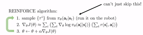
The Policy Gradient Methods try to model a Policy that will maximize the expected Rewards. The Policy $\pi_\theta(a|s)$ is usually learnt by a function approximator- where $\theta$ is the parametrized network.

The Objective is :

$maximize_\theta \mathbb E_{\pi\theta} \left[ \sum_{t=0}^{T-1} \gamma^tr_t\right]$

Maximize the Expected rewards computed from a trajectory , generated by the policy $\pi_\theta$.

To find the best $\theta$ for any function $f(x)$ we need to do stochastic gradient ascent on $\theta$

$\theta \leftarrow \theta + \alpha \triangledown f(x)$

Here $f(x)$ is our sum of rewards objective in our previous equation. so we need to find

$\triangledown \mathbb E_{\pi\theta} \left[ \sum_{t=0}^{T-1} \gamma^tr_t\right] \dashrightarrow (1)$

How to Calculate $\triangledown_\theta \mathbb E \left[ f(x)\right]$

Using Log Derivative Trick

Mathematical expectation, also known as the expected value, is the summation or integration of a possible values from a random variable. It is also known as the product of the probability of an event occurring, and the value corresponding with the actual observed occurrence of the event

So the expected value is the sum of: [(each of the possible outcomes) × (the probability of the outcome occurring)].

The Expectation of $f(x)$ under the distribution $p$

$\mathbb{E}_{x\sim p(x)}\left[ f(x)\right] = \int p(x)f(x)dx$

Expanding for $\mathbb E \left[ f(x)\right]$

$\bigtriangledown_\theta \mathbb E \left[ f(x)\right] = \bigtriangledown_\theta \int p_\theta(x)f(x) dx$

Multiply and divide by p(x)

$\int p_\theta(x) \frac {\bigtriangledown p_\theta(x)} {p_\theta(x)} f(x)dx$

Using the log formulae $\triangledown_\theta log(z) = \frac 1 z \triangledown_\theta z$

$\int p_\theta(x) \bigtriangledown_\theta log p_\theta(x)f(x)dx$

Again rewriting using Expectation:

$\triangledown_\theta \mathbb E \left[ f(x)\right]= \mathbb E \left[ f(x) \bigtriangledown_\theta logp_\theta(x)\right] \dashrightarrow(2)$

We will replace the x with the trajectory $\tau$ .Next step is to find the log probability of the trajectory $\tau$.

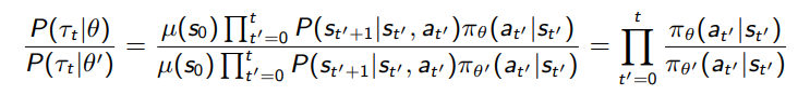
Computation of $log p_\theta(\tau)$

Let,

$\mu$ - starting state distribution

$\pi_\theta$ - Policy - probability of taking an action given a state

P - Dynamics of Environment

Trajectory = Initial State + Further Transitions from the initial state based on actions taken following policy $\pi$.

We can notice that when taking the gradients , the dynamics disappear and thus , Policy gradients doesn’t need to know the environment Dynamics.

$\triangledown_\theta \log p_\theta(\tau) = \triangledown \log \left(\mu(s_0) \prod_{t=0}^{T-1} \pi_\theta(a_t|s_t)P(s_{t+1}|s_t,a_t)\right) \\ = \triangledown_\theta \left[\log \mu(s_0)+ \sum_{t=0}^{T-1} (\log \pi_\theta(a_t|s_t) + \log P(s_{t+1}|s_t,a_t)) \right]\\ = \triangledown_\theta \sum_{t=0}^{T-1}\log \pi_\theta(a_t|s_t)\dashrightarrow(3)$

Objective: $\triangledown \mathbb E_{\pi\theta} \left[ \sum_{t=0}^{T-1} \gamma^tr_t\right]$

Substituting (3) in (2) and then (2) in (1)

$\nabla_\theta \mathbb{E}_{\tau \sim \pi_\theta}[R(\tau)] = \mathbb{E}_{\tau \sim \pi_\theta} \left[R(\tau) \cdot \nabla_\theta \left(\sum_{t=0}^{T-1}\log \pi_\theta(a_t|s_t)\right)\right] \dashrightarrow(4)$

$R(\tau)$ - The reward function that we want to maximize.

The Expectation of the rewards over the trajectory following the policy $\pi$

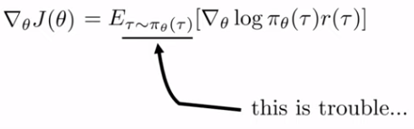
This is the Objective in Policy Gradient problem

As expained in Pong From Pixels

This equation is telling us how we should shift the distribution (through its parameters $\theta$) if we wanted its samples to achieve higher scores, as judged by the Reward Function. It’s telling us that we should take this direction given by gradient of $\log \pi_\theta(a_t|s_t)$ (which is a vector that gives the direction in the parameter space $\theta$) and multiply onto it the scalar-valued score Rewards. This will make it so that samples that have a higher score will “tug” on the probability density stronger than the samples that have lower score, so if we were to do an update based on several samples from p the probability density would shift around in the direction of higher scores, making highly-scoring samples more likely.

We see that the Rewards (scalar values) is multiplied with the Gradient of the Log probability of the action , given state. The Gradient Vector point the direction we should move to optimize the objective. The Gradient is factored by the Rewards.

This enables Probability density function moves towards the action probabilities that creates high score.

Good Stuff is made More Likely.

Bad stuff is made less likely .

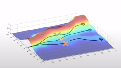
CS285: Trajectories with Good and Bad Rewards

---

As explained in GAE paper, these are some of the variations of this Policy Gradient where the Rewards function is replaced with other expressions for bias Variance Trade-off

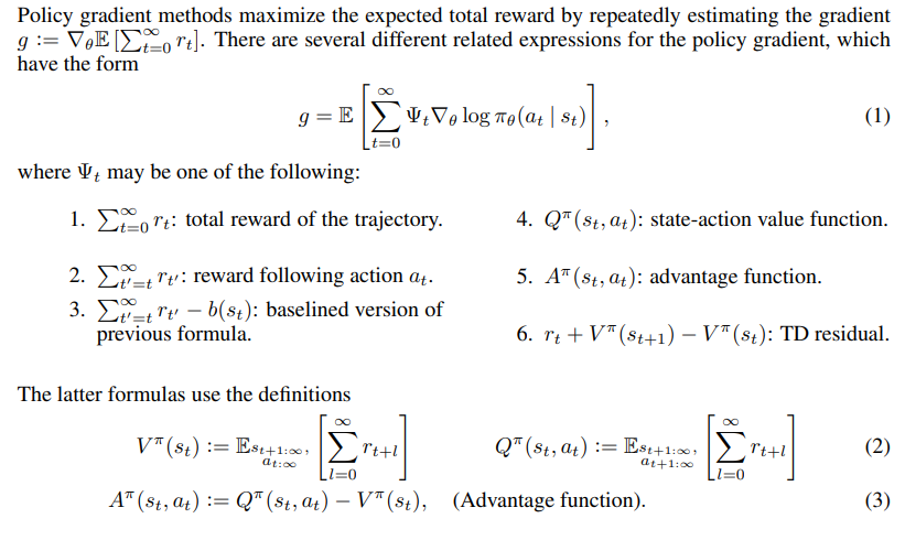
GAE Paper : https://arxiv.org/pdf/1506.02438.pdf

Importance Sampling in Policy Gradients

Policy Gradient is On-Policy - Every time we generate a policy we need to generate own samples

So the steps are

1. Create Sample with the current Policy.
2. Find the Gradient of the objective.
3. Take a gradient step for Optimization.

This is because, The objective is the Expectation of the grad log over the current Trajectory generated by the current Policy .

CS285:https://youtu.be/Ds1trXd6pos?t=3415

Once we take the gradient over the policy , the policy is changed and we cannot use the Trajectory generated previously. We need to new samples again with the current policy.

This is shown below

CS285:https://youtu.be/Ds1trXd6pos?t=3415

What if we don’t have the samples from the policy $\pi_\theta(\tau)$ instead we have $\overline \pi(\tau)$

Importance Sampling comes into play here!

Importance Sampling:

From Wikepdia,

In statistics, importance sampling is a general technique for estimating properties of a particular distribution, while only having samples generated from a different distribution than the distribution of interest.

Expectation of random variable $f(x)$ under distribution $p$ in terms of distribution under $q$

The Expectation of a random variable $f(x)$ under distribution $p$

$\mathbb{E}_{x\sim p(x)}\left[ f(x)\right] = \int p(x)f(x)dx$

Multiplying and dividing by $q(x)$

$= \int \frac {q(x)} {q(x)} p(x)f(x)dx$

Rearranging $q(x)$

$= \int {q(x)} \frac {p(x)} {q(x)} f(x)dx$

This is equal to the Expectation under distribution $q$ given by

$\mathbb{E}_{x\sim p(x)}\left[ f(x)\right]=\mathbb{E}_{x\sim q(x)}\left[ \frac {p(x)}{q(x)} f(x)\right]$

So Expectation under $p$ for $f(x)$ is equal to the Expectation under $q$ with the ratio $\frac {p(x)}{q(x)}$ times $f(x)$

Plugging this for the old policy distribution $\overline \pi(\tau)$, The objective becomes

$J(\theta) = \mathbb{E}_{\tau\sim \overline\pi(\tau)}\left[ \frac {\pi_\theta(\tau)}{\overline \pi(\tau)} r(\tau)\right]$

---

Quick Recap:

The original Objective

$J(\theta) = \mathbb{E}_{\tau\sim \pi_\theta(\tau)}\left[ r(\tau)\right]$

Estimating for the new parameters $\theta$’ with Importance Sampling

$J(\theta)' = \mathbb{E}_{\tau\sim \pi_\theta(\tau)}\left[ \frac {\pi_{\theta'}(\tau)}{ \pi_\theta(\tau)} r(\tau)\right]$ $\nabla_{\theta'}J(\theta)'= \mathbb{E}_{\tau\sim \pi_\theta(\tau)}\left[ \nabla_{\theta'}\frac {\pi_{\theta'}(\tau)}{ \pi_\theta(\tau)} r(\tau)\right]$

Using identity ,$\pi_\theta(\tau)\nabla_\theta log\pi_\theta(\tau) = \nabla_\theta \pi _\theta(\tau)$

$= \mathbb{E}_{\tau\sim \pi_\theta(\tau)}\left[ \frac {\pi_{\theta'}(\tau)}{ \pi_\theta(\tau)} \nabla_{\theta'}log \pi_{\theta'}(\tau)r(\tau)\right]$ $\nabla J(\theta) = \mathbb{E}_{\tau\sim \pi_{\theta_{old}}(\tau)}\left[ \frac {\pi_{\theta}(\tau)}{ \pi_{\theta_{old}}(\tau)} \nabla_{\theta}log \pi_{\theta}(\tau)r(\tau)\right]$

Importance sampling enables us to use the samples from the old policy to calculate the Policy Gradient

Problems with Importance Sampling:

$\nabla J(\theta) = \mathbb{E}_{\tau\sim \pi_{\theta_{old}}(\tau)}\left[ \frac {\pi_{\theta}(\tau)}{ \pi_{\theta_{old}}(\tau)} \nabla_{\theta}log \pi_{\theta}(\tau)r(\tau)\right]$

Expanding $\frac {\pi_{\theta}(\tau)}{ \pi_{\theta_{old}}(\tau)}$

http://rail.eecs.berkeley.edu/deeprlcourse-fa17/f17docs/lecture_13_advanced_pg.pdf

The Policy Gradient Objective with IS and Advantage Function is

$\nabla J(\theta) = \mathbb{E}_{\tau\sim \pi_{\theta_{old}}(\tau)}\left[ \frac {\pi_{\theta}(s_t,a_t)}{ \pi_{\theta_{old}}(s_t,a_t)} \nabla_{\theta}log \pi_{\theta}(s_t,a_t)A(s_t,a_t)\right]$

High Variance in Importance Sampling :

$VAR[X]=E[X^2]-(E[X])^2$

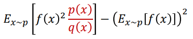
The variance of the Importance Sampling Estimator depends on the ratio $\frac {p(x)}{q(x)}$.

As see in above equation for the ratio $\frac {\pi_{\theta}(\tau)}{ \pi_{\theta_{old}}(\tau)}$, the probabilities are all multiplied and many small differences multiply to become a larger.

This ratio if its large ,may cause the gradients to explode .

This also means , we may need more sample data if the ratio is far from 1.

Unstable Step Updates:

The trajectories generated with the old policy , they may be having the states, that are not that interesting. May be they all have lesser rewards then that of the current Policy.But the new policy is dependent on the old policy

We need to use the old policy and make confident updates when we take a gradient step

step updates options

1. Too large step means, performance Collapse
2. Too small ,progress very slow.
3. The right step changes depends where we are in the policy space

Adaptive learning rate - like Adam - doesn’t work well

So the interesting thing is here that the policies nearer in parameter space differs so much in the policy space.

This is because distance in Policy space and Parameter space are different.

http://rail.eecs.berkeley.edu/deeprlcourse-fa17/f17docs/lecture_13_advanced_pg.pdf

We need to find a policy update, that reflects the underlying structure of the policy space as a function of the parameter space.

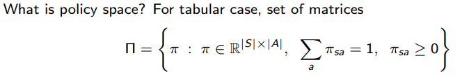
Policy Bounds

Somehow we should bound this difference between these distributions (ie) the Old policy distribution $\pi_\theta$ and new policy $\pi_{\theta'}$ distribution .

We want an update step that is:

• uses rollouts collected from the most recent policy as efficiently as possible
• and takes steps that respect distance in policy space as opposed to distance in parameter space

Relative Policy Performance Bounds:

For this ,we check the performance of one policy to the performance of another policy and check that they are in specific bounds

As explained in this Lecture

We want to produce a new policy update method, which is going to take the form of some kind of optimization problem as in local policy search which is a super class of policy gradient algorithm. We want to maximize some objective, subject to the constraint .. that we are going to say close to the previous policy. So we are going to figure out what that objective is going to be.

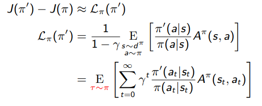
$L_\pi(\pi')$ is our new objective. We call this a surrogate objective.

Now,We can use trajectories sampled from the old policy along with the Advantage calculated from the old policy Trajectory. Still we need the new policy action probability , however we don’t want to rollout for the new policy to collect the rewards.

So what about the constraint/Bounds?

As seen from the above equation, $L_\pi(\pi')$ is the Surrogate Objective. We maximize that surrogate objective , so as to reduce absolute value in the Left hand of the below equation. We do it such a way to keep the KL divergence in some limits.

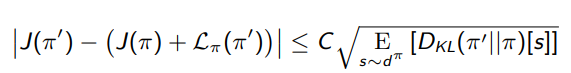
The policies should be bound by KL divergence. If KL divergence of two policies are less, they are close in Policy space

Kullback-Leibler Divergence:

Its a measure of difference between two distributions. The distance between two distributions P(x) and Q(x) given as

$D​_{KL​​}(p∣∣q)=\sum _{i=1}^N p(x_i​​)⋅(log p(x​_i​​)−log q(x​_i​​))\\D​_{KL​​}(p∣∣q)=E[log p(x)−log q(x)]\\D_{KL}(P||Q) = \sum_xP(x)log\frac {P(x)}{Q(x)}$

Its the expectation of the Logarithmic difference between the two probabilities P and Q.

KL Divergence of Two policies $\pi_1\space and\space \pi_2\space$ can be written as

$D_{KL}(\pi_1||\pi_2)[s] = \sum_{a \epsilon A}\pi_1(a|s)log\frac {\pi_1(a|s)}{\pi_2(a|s)}$

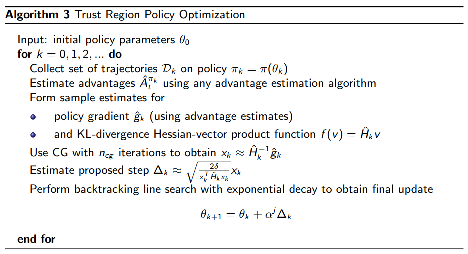
TRPO sneak peak:

The objective is

$\underset{\theta}maximize\ \mathbb{\hat E}_t\left[ \frac {\pi_{\theta}(s_t,a_t)}{ \pi_{\theta_{old}}(s_t,a_t)} \hat A_t \right]$

So,we Maximize the objective , subjecting to condition, the KL Divergence between two policies are less than a value $\delta$. This can be written as

$\mathbb{\hat E}_t\left[ KL\left[ {\pi_{\theta_{old}}(\cdot|s_t)},{ \pi_{\theta}(\cdot|s_t)}\right] \right] \le \delta$

With Lagrangian Dual Trick, we write as unconstrained optimization problem

$\underset{\theta}maximize\ \mathbb{\hat E}_t\left[ \frac {\pi_{\theta}(s_t,a_t)}{ \pi_{\theta_{old}}(s_t,a_t)} \hat A_t - \beta KL\left[ {\pi_{\theta_{old}}(\cdot|s_t)},{ \pi_{\theta}(\cdot|s_t)} \right]\right]$

Here penalty coefficient $\beta$ is constant value,Natural Policy Gradient is used , and additionally the computational Intensive Hessian Matrix has to be calculated.

http://rail.eecs.berkeley.edu/deeprlcourse-fa17/f17docs/lecture_13_advanced_pg.pdf

More details on TRPO in this medium post by Jonathan Hui

Proximal Policy Optimization:

In PPO we try to constraint the new policy near to the old policy but ,without computing Natural Gradient. There are two variants.

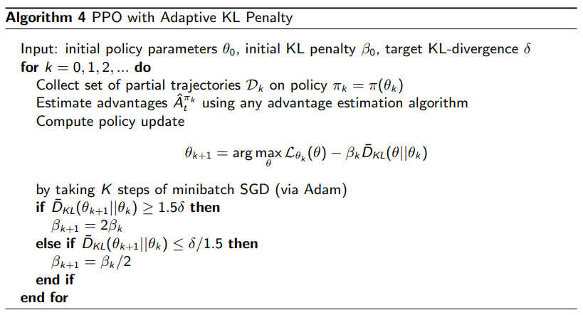
• Adaptive KL Penalty

This solves a constraint problem similar to TRPO. PPO uses a soft penalty coefficient to penalize the KL divergence and its adjusted appropriately over the course of the training. This is a first order method

The Objective is :

$L^{KLPEN}(\theta)= \mathbb{\hat E}_t\left[ \frac {\pi_{\theta}(s_t,a_t)}{ \pi_{\theta_{old}}(s_t,a_t)} \hat A - \beta KL\left[ {\pi_{\theta_{old}}(\cdot|s_t)},{ \pi_{\theta}(\cdot|s_t)} \right]\right]$

TRPO(Primal Dual descence strategy) alternates between update the policy parameters and Lagrange multipliers in the same optimization update iteration .However In PPO we keep the penalty coefficient constant for the whole section of optimization and then afterwards modify it.Compute,

$d = \mathbb{\hat E}_t\left[ KL\left[ {\pi_{\theta_{old}}(\cdot|s_t)},{ \pi_{\theta}(\cdot|s_t)}\right] \right]$

If $d>d_{targ}\times1.5,\beta \leftarrow \beta \times 2$. The KL divergence is larger than the target value . Increase the Penalty Coefficient

If $d<d_{targ}/1.5,\beta \leftarrow \beta/2$. The KL divergence is too small than the target, probably lower the penalty coefficient.

CS294: http://rail.eecs.berkeley.edu/deeprlcourse-fa17/f17docs/lecture_13_advanced_pg.pdf

• Clipped Objective

This is much simpler than PPO with KL Penalty.

As usual , the objective function is :

$\underset{\theta}maximize\ \mathbb{\hat E}_t\left[ \frac {\pi_{\theta}(s_t,a_t)}{ \pi_{\theta_{old}}(s_t,a_t)} \hat A_t \right]$

We define $r_t(\theta)$ as the likelihood ratio

$r_t(\theta) = \frac {\pi_{\theta}(s_t,a_t)}{ \pi_{\theta_{old}}(s_t,a_t)}$

We just want to clip this ratio.

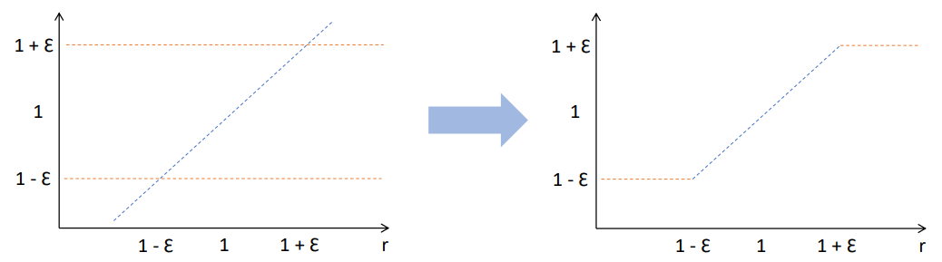
https://cs.uwaterloo.ca/~ppoupart/teaching/cs885-spring18/slides/cs885-lecture15b.pdf

We can see that the ratio r is clipped between $1+\epsilon$ and $1-\epsilon$ where $\epsilon$ is the clipping hyperparameter

The Clipped objective is :

$L^{CLIP}(\theta)= \mathbb{\hat E}_t\left[min (r_t(\theta) \hat A_t , clip \left[r_t(\theta),1-\epsilon , 1+\epsilon \right] \hat A_t )\right]$

We take the minimum between the unclipped value $r_t(\theta) \hat A_t$ and the clipped value $(clip \left[r_t(\theta),1-\epsilon , 1+\epsilon \right] \hat A_t)$. This make the policy update to be more pessimistic and discourages from make abrupt changes in policy updates based on bigger/smaller rewards.

We don’t have any constraints, no Penalties .There is no KL divergence here , its much simpler and the clipping is easier to implement.

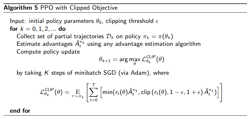
We should note the partial trajectories and the minibatches update for a batch.

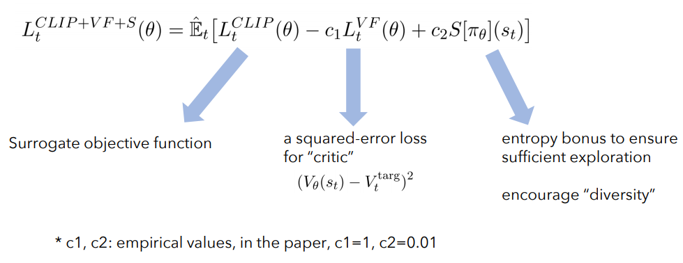
PPO practice:

When we use PPO network in an architecture like Actor Critic , (where Policy is actor and Value is critic ) , we use the following in the objective

1. Clipped rewards(Surrogate Function)

2. Squared Error Loss (Critic)

3. Entropy (To encourage exploration)

https://cs.uwaterloo.ca/~ppoupart/teaching/cs885-spring18/slides/cs885-lecture15b.pdf

PPO Implementation:

There are many github repositories that has PPO implementation. There is one from openai/baselines ,famous pytorch implementation by ikostrikov , QunitinFettes, CleanRL , higgsfield/RL-Adventure etc..

There is a nice blog post on PPO Implementation details .Please check this list for your implementation details.

I have implemented a PPO Notebook for continuous environment with the boiler plate code provided by Yandex. My implementation may not be perfect.

I will just highlight few items here.

Network Architecture:

Its suggested to use Orthogonal initialisation with parameter $\sqrt2$ and biases zero.

def layer_init(layer, std=np.sqrt(2), bias_const=0.0):
    '''
    https://github.com/vwxyzjn/cleanrl/blob/
    418bfc01fe69712c5b617d49d810a1df7f4f0c14/cleanrl/ppo_continuous_action.py#L221
    '''
    nn.init.orthogonal_(layer.weight, std)
    nn.init.constant_(layer.bias, bias_const)
    return layer

The network is kind of Actor critic,wherein we use one network for policy and another one for values. The activation function is tanh.

class Model(nn.Module):
    def __init__(self,num_inputs,num_outputs):
        super(Model,self).__init__()
        self.fc1 = layer_init(nn.Linear(input_shape,64))
        self.fc2 = layer_init(nn.Linear(64,64))
        self.fc_Policy = layer_init(nn.Linear(64,n_actions))
        self.fc_Value = layer_init(nn.Linear(64,1))
        self.covariance = nn.Parameter(torch.zeros(1,n_actions))
        
    def Policy_network(self,x):
        '''
        The network predicts the mean and covariance(log of standard deviation)
        '''
        x = torch.tanh(self.fc1(x))
        x = torch.tanh(self.fc2(x))
        mean = self.fc_Policy(x)

        logstd = self.covariance.expand_as(mean)
        return mean,logstd
    
    def Value_network(self,x):
        '''
        The network predicts the Value Function
        '''
        x = torch.tanh(self.fc1(x))
        x = torch.tanh(self.fc2(x))
        x = self.fc_Value(x)
        return x

This Model is wrapped with another Class Policy to call in the Model in two different conditions

1. When in Collecting partial Trajectories

   This is called partial trajectories as we wont collect the trajectory until the end. But we just collect a fixed set of tuples {actions, log_probabilities,values} for the policy

if not training:
        '''
        training=False -- Value
        Input is Observation 
        Sample action for a Trajectory
        return {"actions:","log_probs","values"}
        '''
        with torch.no_grad():
            x = torch.Tensor(inputs).unsqueeze(0)
            mean,logstd = self.model.Policy_network(x)
            std = torch.exp(logstd)
            distrib = Normal(mean,std)
            action = distrib.sample()[0]
            log_prob = distrib.log_prob(action).sum(1).view(-1).cpu().detach().numpy()
            value = self.model.Value_network(x).view(-1).cpu().detach().numpy()
        return {"actions":action.detach().numpy(),"log_probs":log_prob,"values":value}

1. When in training

   Just return the action distribution along with the values. This will be called when making every step update.

else: 
        '''
        training=True - - Policy & Value
        
        Input is Observations
        return {"distribution","values"}
        '''
        x = torch.Tensor(inputs)
        mean,logstd = self.model.Policy_network(x)
        std = torch.exp(logstd)
        distrib = Normal(mean,std)
        value = self.model.Value_network(x)
        return {"distribution":distrib,"values":value}

Generalized Advantage Estimate GAE:

We use an Advantage Estimator that has two parameters $\gamma \space and \space \lambda$ for bias-variance trade off as explained in GAE paper

We initialize all the values first .

We have the last observed state in the Trajectory . To get the values for that last state, we call the Network model

    advantages = []
    returns =[]
    lastgae = 0
    rewards = trajectory["rewards"]
    values = trajectory["values"]
    dones = 1- trajectory["resets"]
    
    #Get the latest state
    last_state = trajectory["state"]["latest_observation"]
    # Output of the network for the 'next_state' input
    network_output  =self.policy.act(last_state, training=False)
    last_value = network_output["values"]
    values = np.append(values,[last_value])# Append the next  value

Next , we loop through to calculate the Advantage. We calculate the returns as advantage+values

# https://github.com/colinskow/move37/
# blob/f57afca9d15ce0233b27b2b0d6508b99b46d4c7f/ppo/ppo_train.py#L69
  for step in reversed(range(len(rewards))):            
      td_delta = rewards[step] + self.gamma * values[step+1] * dones[step] - values[step]
      advantage =lastgae= td_delta + self.gamma*self.lambda_*dones[step]*lastgae
      advantages.insert(0,advantage)
      returns.insert(0,advantage+values[step])

Losses

Policy Loss

The clipped objective is

$L^{CLIP}(\theta)= \mathbb{\hat E}_t\left[min (r_t(\theta) \hat A_t , clip \left[r_t(\theta),1-\epsilon , 1+\epsilon \right] \hat A_t )\right]$

Advantage is calculated from old policy. Ratio is calculated between new policy and old policy.

def policy_loss(self, trajectory, act):
    """ Computes and returns policy loss on a given trajectory. """
    
    actions = torch.tensor(trajectory["actions"]).to(device) 
    old_log_probs = torch.tensor(trajectory["log_probs"]).to(device).flatten() 
    new_distrib = act["distribution"] 
    new_logprobs = new_distrib.log_prob(actions).sum(1)
    entropy = new_distrib.entropy().sum(1)
    self.entropy_loss = entropy.mean()

    
    ratio = torch.exp(new_logprobs - old_log_probs)
    surrogate1 = ratio * -torch.Tensor(trajectory["advantages"]).to(device)
    surrogate2 = torch.clamp(ratio,1-self.cliprange,1+self.cliprange)*-torch.Tensor(trajectory["advantages"])
    policy_loss = torch.mean(torch.max(surrogate1,surrogate2))
    return policy_loss

Value Loss:

We use clipped value loss function.

def value_loss(self, trajectory, act):
    """ Computes and returns value loss on a given trajectory. """
    new_values = act["values"].flatten() 
    # returns(Target Values)= Advantage+value
    returns = torch.tensor(trajectory["value_targets"]).to(device) #Advantage+value
    old_values = torch.tensor(trajectory["values"]).to(device).flatten() # Old Values
    # Squared Error Loss
    v_loss1  =(returns - new_values ).pow(2) # Target_values - New_values
    clipped_values = old_values+ torch.clamp(new_values - old_values,-self.cliprange,self.cliprange)
    v_loss2 = (clipped_values - returns ).pow(2) # Target_values - clipped_values 
    
    value_loss = 0.5*(torch.max(v_loss1,v_loss2)).mean()
    return value_loss

Total Loss:

total_loss = policy_loss + self.value_loss_coef * value_loss - self.entropy_coef*self.entropy_loss

Helpful Blogs:

1. https://spinningup.openai.com/en/latest/algorithms/ppo.html

2. https://lilianweng.github.io/lil-log/2018/04/08/policy-gradient-algorithms.html

3. https://danieltakeshi.github.io/2017/03/28/going-deeper-into-reinforcement-learning-fundamentals-of-policy-gradients/

4. https://cs.uwaterloo.ca/~ppoupart/teaching/cs885-spring18/slides/cs885-lecture15b.pdf

5. http://rail.eecs.berkeley.edu/deeprlcourse-fa17/f17docs/lecture_13_advanced_pg.pdf

6. Expectation
7. Pong from Pixels

Video Tutorials:

1. CS 285 - Berkley Deep RL Lectures especially this on TRPO and PPO
2. PPO from CS 885 Waterloo Deep RL course .
3. Coding Tutorial from schoolofai